

One of the most common requests I hear from colleagues and customers is, “How do I estimate how many jobs I can run on a node and how fast will they run?” The immediate and most accurate answer is… it depends. While it may seem a flippant answer, it is a succinct response to a complex multidimensional problem. Let’s examine the variables.
Starting with the sources, different sources will “serve up” the data at different rates. Reading a file from a remote sftp site is going to be slower than reading from a local database. SaaS applications also vary in their response time due to load. Also, the further away the source is, the greater the chance of different routing. One set of packets may arrive via Cleveland, and another set may come through New York City. The first set of variables are the source and the network.
Once the data “arrives” at the node, the Snap converts whatever the source form is into a JSON document. Each row of data, SOAP message, JSON document or whatever form the data is, has a size that can vary widely. When we were working with relational databases, the size of a row of data would not exceed the total number of columns times bytes in the result set. Today, payloads can range from a couple hundred bytes to megabytes within the same request. This wide range of size makes it difficult to accurately measure performance and memory requirements. And unlike databases where there is a set upper limit, there is no set upper boundary with poly-structured sources.
The response to a request, network latency, and data size can vary widely. However, the amount of memory and processing speed of the JVM is static. A node is a server, real or virtual, running a Linux or Windows OS. In the case of a Cloudplex, it is managed by SnapLogic and is consistent because we use a standard image for all plexes. Groundplexes are setup by customers and as such have the potential for different performance metrics due to system and network configurations. This can change behavior from one location to another.
Essentially, there are two types of Snaps: streaming and accumulating. Streaming snaps receive a JSON document, process it and pass it on to the next snap. There is only one document in the Snap at any time. Accumulating Snaps are the reverse, the incoming data is stored in the Snap until the entire data flow has been consumed. There are not many accumulating Snaps and they are easy to identify. If the operation you want to do is acts upon more than one document, it is an accumulator. The Sort Snap is the most obvious. The amount of memory and disk required is dependent on the number of documents and since they can vary widely it is difficult to be exact. While SnapLogic attempts to do everything in memory like Spark, it will overflow to disk when required. The means the node needs to have enough disk space to handle these conditions. Estimated memory requirements include both RAM and disk space.
When a pipeline is started, the control plane sends the Snaps to a node on the plex. When it is instantiated, each Snap has a memory footprint. The size of Snap can vary widely, and some like the SAP Snap have external dependencies that have to be factored into the requirements. Also Snap sizes can change from release to release as we make improvements, add features or update to APIs or infrastructure changes. Some changes will reduce the memory footprint, others will increase it. The only constant is change.
Finally, the data needs to be delivered to the target or targets. Just like the variations we have with input, the network and target behavior can vary widely. Source and target performance can be thought of two sides of the same coin. The only difference being the conditions that influence the performance of the source may or may not be the same as the target. You can have a source that can serve up the data much faster than the target can consume it. The reverse can happen, and that is usually not something you can influence.
So is it impossible to accurately know the memory requirements and performance characteristics of an integration job? Yes, but when you can’t be exact, you estimate. You can define a range of requirements and behavior knowing there will be “outliers” based on conditions beyond your control.
SnapLogic provides the ability to monitor pipeline characteristics in the dashboard.
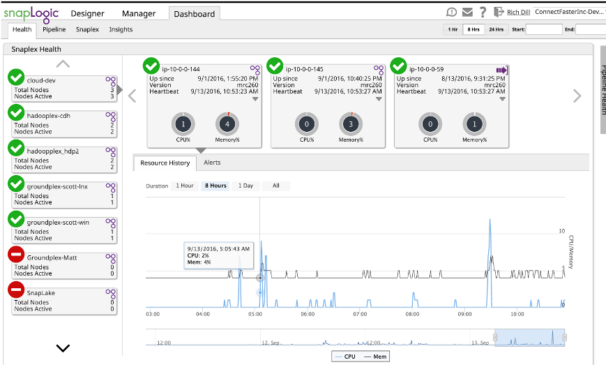
Using the Dashboard, combined with a series of test runs, you can develop a sense of memory and performance requirements. Simply run the pipeline and use the Dashboard to see the memory used. While it is given as a percentage, if you know the memory of the node it is a simple “problem for the student” to convert it to actual memory used. Detailed memory usage and performance is in the log file of each run. These logs provide Snap by Snap memory and performance information that can be used not only for estimating, but also tuning. But that’s another blog post.
Integration today happens in an environment with many variables outside the control of the user. We need to have realistic expectations of performance and behavior. The loosely coupled architecture of SnapLogic provides resilience to change, not only to sources and targets, but runtime conditions as well. You can leverage this powerful capability if you understand how to use to your advantage.
Rich Dill is a SnapLogic Enterprise Solutions Architect. He was recently featured on our podcast series SnapTalk discussing the lifecycle of data.